- HOME
- PRODUCTS & SERVICES
GIS/GPS in Smart Cities/Transport METRIS — Big Data in Metro Transportation METRIS LiveQ: Real-time Truck Queues METRIS — Port Performance METRIS — GPS Tracking METRIS — Transport Planning Advanced GIS Analytics/Algorithms Transport Research Error Modeling Conflation GIS in Retail CLEO — Location Optimization Trade Areas Gravity Models Location-Allocation Models Enterprise GIS Strategic plan & cost-benefit analysis GIS Data Modeling
- RESOURCES
News & Commentary METRIS News & Press Reports Light Technical Geography 80-20 (nuggets for adults) Geography Kids' Hangout Technical GIS Publications METRIS Publications Associated projects NCRST VITAL
- ABOUT
Conversational UTM
Val Noronha | The Geography 80-20 collection
The Universal Transverse Mercator (UTM) grid appears on some topo maps, off at a slight angle to the border rectangle. It is a mathematically advanced projection, used mostly by professional geographers and the military, to run precise measurements and analyses on maps. But users are shielded from the math; to us it's just a standard (x,y) coordinate system for the earth. Obviously (x,y) can't work on a sphere, so the UTM approach is to have subsets of the earth behave as flat surfaces. In fact many projections do that; what sets UTM apart is that it supports high accuracy, and that it's easily standardized globally.
Generally speaking, anybody can treat a topo as an (x,y) coordinate system: set up a square grid on a tracing sheet, take measurements and run analyses. But that coordinate system can't be related back to the global lat-long system. Using UTM it can.
UTM Grid References
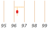
 A first
concept we have to master with any grid system is interpolating
and expressing coordinates. The shed in the map is between 96
and 97, about a third of the way up the interval. So we figure
it's 96.3, and print it without the decimal, as 963. That's our
easting. Similarly
we can interpolate a northing
in the map below: 22.8, written as 228.
A first
concept we have to master with any grid system is interpolating
and expressing coordinates. The shed in the map is between 96
and 97, about a third of the way up the interval. So we figure
it's 96.3, and print it without the decimal, as 963. That's our
easting. Similarly
we can interpolate a northing
in the map below: 22.8, written as 228.
The grid coordinate for the shed is therefore 963228: "first easting, then northing,” or more simply and intuitively, x and y. In an operational scenario, an aerial rescue team would scan an area, spot an item of interest, and relay it to a ground crew in this format.
Caution: On some maps there's a set of regularly spaced, roughly vertical lines, inclined slightly off north. They indicate magnetic north, to help orient the map with a compass. A UTM grid has both north-south and east-west grid lines. The inclination of magnetic north lines and the inclination of the UTM grid are entirely unrelated.
That's it! For many basic needs that's all there is to the practical side of using UTM. This article could end right here. If you'd like to know more, read on. Next we'll get into the technical background and design, so that you can relate grid references on one map to those on a neighboring sheet.
A Global Grid
On closer examination of a topo map, we find superscripted
numbers by the principal grid annotations.
On the northings, the 20000
indicates that the numbers 21, 22, etc are abbreviations; they
stand for 21,000 meters, 22,000 meters, etc. So the grid squares
are at 1 km intervals, and our grid reference 963228 above
therefore has an effective precision of 100 meters (1/10 of a
grid interval). That's good to know.
Also on the northings, the 4720 indicates that the y coordinate is 4,720 km from somewhere — the equator. The 396 on the easting similarly indicates that the x coordinate is 396 km from somewhere. Nowhere in particular, actually.
A third item to note is probably in the publication notes in the
legend: Universal Transverse Mercator (or UTM) zone followed by a
number between 1 and 60. If the zone number on two different maps
is the same, and they're in the same N-S hemisphere, even if they're
500 km apart, you can run math (e.g. use the Pythagorean formula to
calculate distance) on the full-length UTM coordinates. You can calculate
differences in bearings among points, though bearings on the UTM grid are not the same
as bearings relative to true north or magnetic north. Getting to the
bottom of all this requires that we examine the design
of this projection.
Background: the Mercator Projection
 A map projection is an attempt at the impossible
task of representing a 3D earth in 2D. It is necessarily a
compromise. Some projections represent distance correctly in
this or that direction, but not shape or area. Others represent
area correctly but not distance.
A map projection is an attempt at the impossible
task of representing a 3D earth in 2D. It is necessarily a
compromise. Some projections represent distance correctly in
this or that direction, but not shape or area. Others represent
area correctly but not distance.
The Mercator Projection is widely used for world maps. It
famously distorts size, e.g. making Greenland look larger than
Africa (in reality Greenland is 7% the size of Africa). It
caused consternation during the Cold War because it made the
Soviet Union appear enormous compared with Europe and the U.S.
This distortion is actually Mercator's solution to the general problem that all cylindrical projections share. At higher latitudes, the map surface (the cylinder) gets further from the globe it represents, and something has to give: distance, area or shape. Mercator sacrifices distance and area to preserve shape — the ratio between a degree of latitude and a degree of longitude. That important property makes it appropriate for use with a mariner's compass, hence it's useful for global navigation.
The flip side is that along the equator, cylindrical projections have zero distortion, because there's no separation between the cylinder and the globe, no geometric transformation. Now suppose we could turn that cylinder 90° and wrap it around a meridian instead, then that meridian would be faithfully represented, and the area immediately around it minimally distorted. We could do that to any meridian, producing a true representation of any part of the world. If we then applied Mercator math to the surroundings, we'd have shape conformity. And by keeping those surroundings quite small, we could put a lid on the worst-case distortion, and be able to measure distances, bearings, everything, with minimal error. This is the concept behind transverse Mercator projections.
Universal Transverse Mercator Grid
![]()
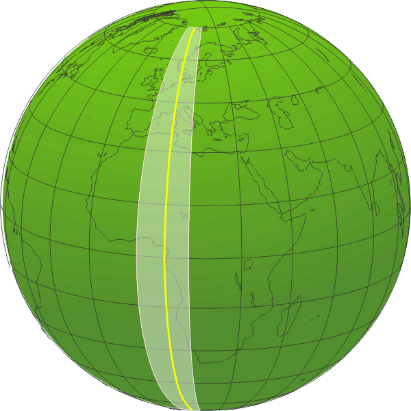
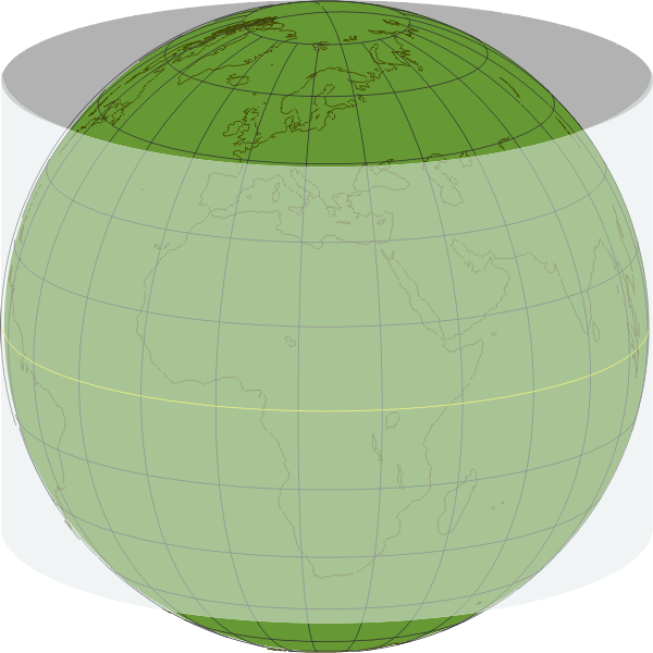
Think about
a giant sheet of regular square graph paper, calibrated in
meters, printed on rigid metal foil, and wrapped around the
earth as shown. It makes contact along a circle, one half of
which is a meridian, which we'll call the central meridian (CM),
the yellow semi-circle (the illustration shows it in the 0°–15°E
range, but it can be anywhere). The cylinder is now trimmed to a
width of 3° of longitude on either side of the CM, for a total
of 6° (a very narrow strip at the global level; the
illustrations show it 15° wide for clarity). Within this 6°
zone, the projection of the earth on to the grid is very
accurate, not 100% (one's a sphere, the other's a plane bent
into a semi-circle), but better than with any other projection,
and the UTM calculations take into account the ellipticity of
the earth and a bunch of other factors.
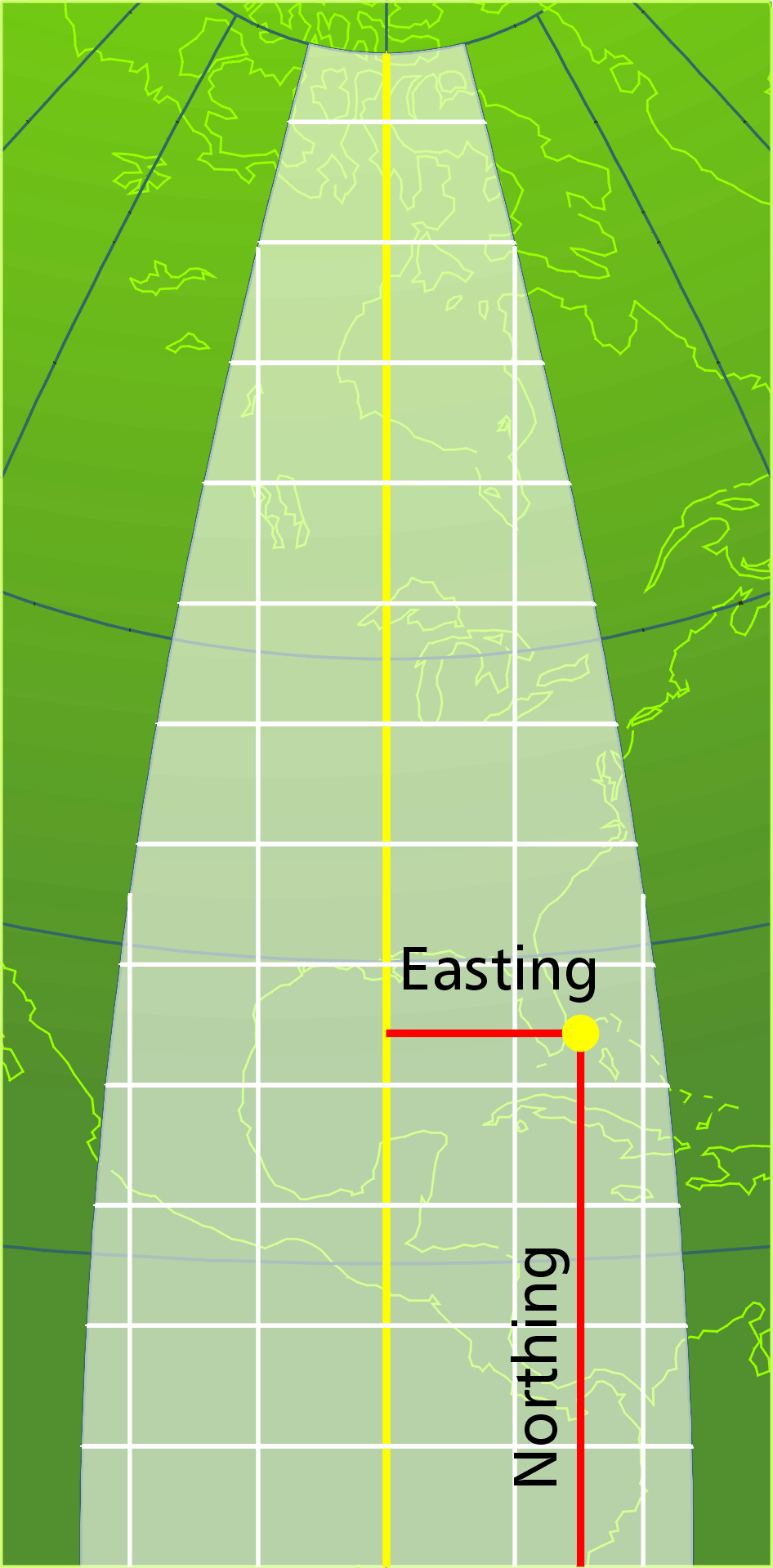 UTM
coordinates are measurements taken off this square grid, which
is entirely distinct from parallels and meridians. For example,
the meridian neighboring the CM converges with the CM at the
pole (in the illustration, the black lines converge). Whereas on
the projection, because it's a standard square (x,y) coordinate
system, if we start at a point neighboring the CM at the
equator, and move “north” on the grid, we're on a path parallel
to the CM and never converge (the white lines).
UTM
coordinates are measurements taken off this square grid, which
is entirely distinct from parallels and meridians. For example,
the meridian neighboring the CM converges with the CM at the
pole (in the illustration, the black lines converge). Whereas on
the projection, because it's a standard square (x,y) coordinate
system, if we start at a point neighboring the CM at the
equator, and move “north” on the grid, we're on a path parallel
to the CM and never converge (the white lines).
That clearly means that the projection grid is not aligned with north, except at the CM. This leads to the third common version of north. To enumerate them all, they are: (a) true north, the orientation of the black-line meridians, (b) magnetic north, where a compass needle points, and now we have (c) grid north, the orientation of the vertical white lines. The deviation among these can be as much as 20°. Topos are produced with true north pointing up. Consequently the UTM grid is inclined at a small angle on topos.
Bottom line: The UTM grid is a Cartesian coordinate system within a 6° longitudinal window of the globe. All measurements are in meters, so the numbers tend to be large, but we can mentally process them into kilometers if more convenient. The great bit about UTM is that we're not subject to that funny mental math about a degree of longitude varying with latitude, and we don't work in degrees measured at the center of the earth. We work in meters in x and y on the earth's surface. The advanced math is in relating UTM coordinates to lat-long, but we don't have to worry about that, computers work it out.
False Easting and False Northing
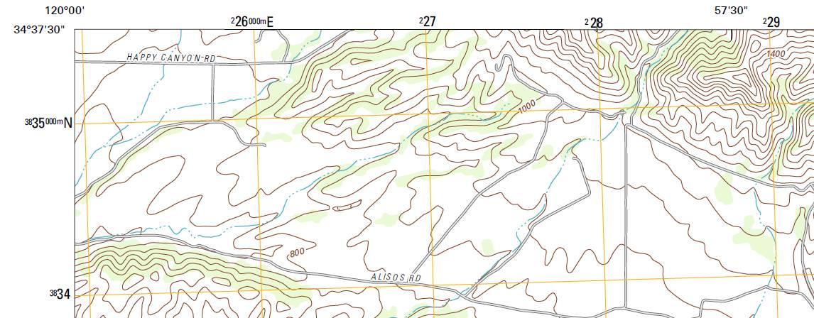
Test your newly learned gnowledge of UTM on this USGS topo extract. Click on it to view it at full size first. Note the UTM grid overlay in orange, and the graduation marks in the margin, both lat-long and UTM.
Eastings and northings should never be negative; we don't want
confusion over whether a point 1 west of 12 is 11 or 13: it
should always be 11. To eliminate any negative x, a false easting of 500,000 m
is added to all eastings, and this value (500K) therefore becomes the
x-coordinate of the CM. A point 100 km west of the CM is not
–100,000 but 400,000 E.
Back to the grid reference exercise above, the 396 is 396,000 m E, meaning we're 396,000–500,000=–104,000: 104 km west of the CM. What are we 396 km east of: in other words, what's the E-W origin of the coordinate system? [Shrug.] On eastings the “zero” line is really the CM, even if it's re-labeled 500K. The new zero is some place west of the zone boundary. Irrelevant.
The equator is designated as 10,000,000 meters north, a false northing, but this applies only to points in the southern hemisphere, so a point 4,000 km south of the equator has a northing of 6,000,000 meters. A point 6,000 km north of the equator also has a northing of 6,000,000 meters. To manage duplicate coordinates, there's a system of zones.
UTM Zones
UTM is set up as 60 projection zones, each like the strip illustrated above, beginning at 180°W, and stepping eastward in 6° intervals. The first strip is Zone 1, extending from 180°W to 174°W with a CM at 177°W. Zone 2 is 174°W to 168°W with a CM at 171°W, etc. This takes care of multiple instances of 396,000 m E. But there's still potential for ambiguity because places in the northern and southern hemisphere can have the same northings. So the hemisphere should become part of the location spec: to place any point on the earth unambiguously, we'd need: {zone, hemisphere, easting, northing}, e.g. 11 N 326809, 4318679 where N is the northern hemisphere. This notation is used by some researchers but it is not the official UTM syntax.
There's an alphabetic scheme of labeling latitudinal sections,
in 8° intervals: beginning with zone C at 80°S to 72°S, and
stepping north, skipping letters I and O. The first northern hemisphere
zone from 0°N to 8°N is N, the second from 8°N to 16°N is P (skipping O), and
it ends at zone X at 72°N to 84°N (a special 12° zone). Zones A
and B cover the South Pole area, zones Y and Z cover the North
Pole area. Since there is no ambiguity in northing between say
23°N and 63°N, the latitudinal zoning scheme does not clarify
anything by labeling one Q and the other V. Being redundant, it
can serve as a range check on the northing. The official UTM
location syntax is {E zone, N zone, easting, northing}, e.g. 11 S 326809, 4318679
where S is not the southern hemisphere but the 32°N to 40°N
latitudinal zone in which this point falls. Clearly there's a danger in using the
unofficial hemisphere expression above, because S in particular can conflict with
the official syntax and point to a different place.
The polar areas north of 84°N and south of 80°S are covered not
by UTM but by a Universal Polar Stereographic (UPS) projection.
GPS and UTM
Given all the merits of UTM, why don't GPS units report UTM and let us work in meters rather than lat-long degrees? Most dedicated GPS receivers do, but some older consumer devices don't, or you have to go through the setup menu to turn it on. UTM is great for accurate work on large-scale (high magnification factor) maps: tactical military ops, urban analysis, construction, hiking. It's not designed for global applications where we have to work across zones. The concepts in which UTM is framed are a bit involved. There are some practical gotchas, as when a city or state straddles zone boundaries. Professionals who use UTM on a regular basis have software that translates between lat-long and UTM easily, but occasional map users tend to find latitude and longitude, with all its 3D geometric complexities, easier to grasp.

Tweet this URL
© Digital Geographic Research Corporation Contact us